AIRFOIL PRIMER

FOR

NON-AERODYNAMICISTS

JOHN DREESE

DREESECODE SOFTWARE LLC

RED HOPE

Pages: 30

No part of this book can be reproduced in any form by any means without the express permission of the author. This includes reprints, excerpts, photocopying, recording, or any future means of reproducing text.

Email: DesignFOIL@gmail.com

Web: http://www.dreesecode.com/primer/

Twitter: http://www.twitter.com/JJDreese/

Amazon Kindle Version available from:

http://www.amazon.com/dp/XXXXXXXX

Version 1.0

Published in the United States of America.

PREFACE/FIGURE NAMES

This book is the culmination of a five-part magazine article series that I wrote in 2004. It is one of the most popular features on the DesignFOIL website and I’ve been asked to put it in a simple Kindle format for people to read offline.

Figures: On the website, each part is a standalone web page and the figure numbers refer to that web page. In this Kindle book all five web pages are combined – each one is a chapter. The figure names refer to that particular chapter. So you might see a reference to Figure 2. It means Figure 2 from –that- chapter.

Regards,

John Dreese

NOTE:

All airfoil shapes and data were created using DesignFOIL. A free demo is available on the website at www.dreesecode.com

PART 1:

WING SECTIONS & LIFT

Airshows are a great place to study airplanes and crowd psychology. We wait patiently in long lines for hotdogs, bathrooms and overpriced water. Of course, people do that at all large gatherings, but the one group activity found only at airshows is the creation of the people-filled shadows, as shown in Figure 1.

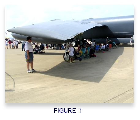
As the hot Sun cooks the crowd, they migrate under the protective wing shadows of huge airplanes, preferably a C-130 or a B-52 bomber; something with a huge wing area. And just like that, we’ve discovered yet another practical use for airplane wings!

This primer talks about why we have wings at all. As the aerodynamicist Jack Moran said, wings are simply a thrust amplifier. Sure, we could use rockets to get from point A to point B, but that would be incredibly inefficient as far as fuel usage goes. That’s where wings come in. They provide a similar ability to defy gravity, but at a fraction of the fuel usage compared to rockets.

Rather than use directed raw force, wings have a unique characteristic; they generate a force that is perpendicular to the direction of movement. Airplanes move horizontally, but wings push up vertically (LIFT). This magic of physics is simply a result of how air flows over the wings. This primer series is about how lift is created, how to estimate it, and how to make it happen.

The origin of lift is very simple: it is the result of having lower air pressure above the wing than below it. Air cannot impart direct forces on a wing like a hammer can. Instead, it can only impart forces via two methods: pressure and friction. Those are the only two ways. Lift comes from a pressure difference between the upper and lower wing surfaces. Pretty simple eh?

No doubt, there are many theories as to what causes the required pressure difference. That's where people get all bent out of shape. Blame it on Bernoulli? Blame it on momentum transfer? The devil is in the details.

Streamlined wings aren't the only things that can create lift; a sheet of plywood can also generate lots of lift. Unlike a wing, of course, a sheet of plywood is aerodynamically very inefficient. The secret to making this pressure-difference miracle more efficient is to use a cross-sectional shape that won’t cause separation at the nose. Plywood has a sharp leading edge which generates oodles of DRAG; that's the retarding force that keeps us from moving forward as fast as we’d like to. 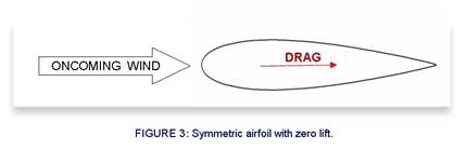Historically, good wings use cross-sectional shapes that are round in the front and sharp in the back. We call this shape an Airfoil (Figure 2). There are parts of the world that use different names like aerofoil and profile.

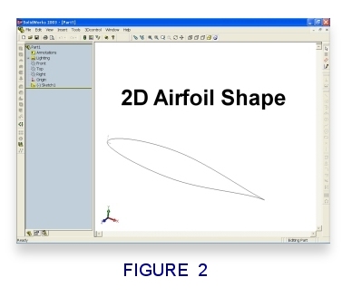
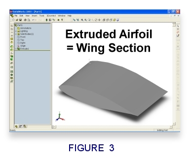
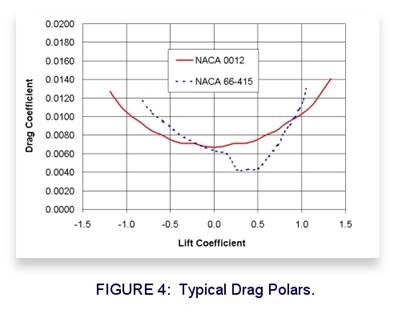
Technically, airfoils are flat two-dimensional shapes, and can’t produce any lift at all; great for pictures on paper, but lousy for lift. You have to extrude an airfoil into the 3rd dimension to create an object that will make lift. We call this extruded shape a wing section (see Figure 3).

So now you have a device that generates a pressure difference, resulting in a vertical lift force and a slight down-deflection of air behind it. Who cares? Millions of airline passengers care.

Nature will direct the airflow around a wing section so that the air obeys the conservation laws of mass & momentum. If the real world physics are obeyed, some of the oncoming air will go over the wing section and some will go under the wing section. The point on the leading edge where the oncoming flow splits is called the stagnation point. Strangely enough, the velocity of air at that very point is zero. There's another stagnation point at the trailing edge, where these two travelling air masses come back together. Figure 4 illustrates these stagnation points.

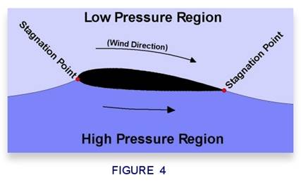
The air pressure along the upper and lower surfaces can vary wildly. It usually drops lower than ambient pressure along the upper surface, especially if the wing section is angled up at all. For a lifting airfoil, the airflow above is typically accelerated faster than the air below. Think of it as the air up front racing fill the void of all that air you just pushed down behind the wing. From Bernoulli's famous effect, we know that when air speeds up, the air pressure drops. The end result is that the pressure difference between the lower and upper surface literally sucks the wing upward!

To conclude the idea, lift comes from a combined effort of the wing being sucked upwards and the wing deflecting some of the air downward. The effects are so intrinsically linked together that we can calculate the lift force by simply measuring surface pressures around the wing section. That's one method which wind tunnels use to measure lift forces and pitching moments on a wing section model. Many advanced wind tunnels use a different technique for drag which measures how much momentum the model "steals" from the oncoming airflow via the boundary layer; we'll get into that later.

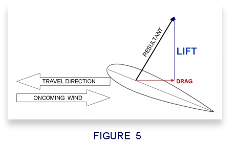
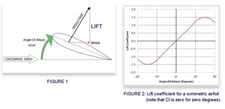
One last note about lift. A wing section exposed to an oncoming wind generates a single united force, usually pointing up vertically and slightly backwards. We call this theResultant force. Lift is the portion of that force that is perpendicular to the direction of travel, not the direction the airfoil is pointing. Drag is the portion that is parallelto the direction of travel. See Figure 5 for an illustration.

Now you know where lift comes from. Next time, we'll learn the basic terms regarding airfoil geometry.

PART 2:

BASIC AIRFOIL GEOMETRY TERMS

Subsonic airfoils should be round in the front and sharp in the back. A century of visual reminders should make this obvious. However, I see it violated often with regard to after-market wings people install on their cars. The wings are already not very effective for the speeds that most cars are driven, but they are -really- ineffective when mounted backwards. Remember: put the round end upstream and the sharp end downstream. That's really the big rule at the core of standard airfoil setup. Everything else is just tweaking and optimization. For our purposes, all airfoil diagrams shown in this primer series assume air movement from left to right.

Let's look at an example:

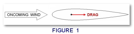
Take a symmetric airfoil and point it directly into the oncoming wind as shown inFigure 1. Since the airfoil is parallel with the wind, we can’t measure or feel any perpendicular forces (up or down in this case). The lift is zero. However, there is a slight tugging force from the friction of air dragging along the airfoil surface. We call this force drag.

You might wonder what use could come from a symmetric airfoil oriented parallel to the wind? It makes for a perfect streamlined fairing, a shield that hides some underlying non-streamlined structure like a wire, antenna, pipe, or landing gear strut.

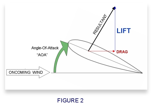
Streamlining is nice, but we want lift. Let’s gently tip the airfoil up to some small angle as shown inFigure 2. Suddenly, there is a noticeable force upwards while the dragging force increases slightly. What you’ve just discovered is that an increase in the angle between the chordline of the airfoil (an imaginary straight line stretching between leading edge and trailing edge) and the oncoming wind will increase the lifting force. This variable angle is called the Angle-Of-Attack, or AOA for short. What you need to know is that increasing the AOA will increase both the lift force and the drag force. This effect will continue up until about 15 degrees. After that, the lift force will start to fall, but drag will continue to grow. We call this phenomenon stall. It is the result of the formerly smooth air over the wing breaking down and separating from the wing. One special note: if the airfoil has upward bow to the shape (camber), then increasing the angle-of-attack may actually decrease the drag force for a few degrees before it resumes its quick climb.

Angle-Of-Attack is the angular difference between where the wing is pointing and where it is moving. The first time I truly understood this was when, as a kid, I saw a Boeing jet climbing very slowly away from Columbus International Airport in Ohio. It appeared to be just plowing through the air nose-high. The airplane nose will not always point straight in the direction the airplane is flying, especially during landing and takeoff.

Figure 3 shows a typical airfoil geometry with the important components labeled. The Upper Surface is the wing section skin on top, from the leading edge to the trailing edge. The Lower Surface is the bottom wing section skin that goes from the leading edge to the trailing edge. Mentioned already is the chord line, which is an imaginary straight line between the leading edge and trailing edge; this is used for measuring/setting Angles-Of-Attack (see Figure 2).

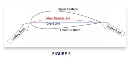
The chord line should not be confused with the mean camber line, or meanline for short. The mean camber line is an imaginary line that divides the airfoil into equal (roughly) upper and lower halves. On a symmetrical airfoil, the mean camber line is thesame as the chord line. However, if you bow the airfoil upwards, you are adding "camber" to the airfoil. A unique characteristic of airfoils with camber is that they produce lift at zero degrees Angle-Of-Attack. The more camber, the more lift. Of course, there is an associated cost of more drag and more pitching moment (we'll get to that later) as well.

A perfect airfoil would allow you to change the mean camber during flight; providing ample camber for takeoff and landing, but very little during cruise. Fortunately, there is a simple method for doing this without resorting to bending or flexing the structure. Instead, we droop down the aft portion of the wing section using a hinge. This device is called a flap and temporarily adds camber to the wing section. Flaps allow our wing section to have lots of camber during takeoff and very little camber during cruise. If the flaps also extend backwards while they droop, then they also provide increased wing area, making for an amplified lifting effect.

In Part 3 of this primer series, we will discuss lift and drag calculations in more detail. We will discuss their respective coefficients, which allow us to compare the performance of different airfoils on a common scale.

PART 3:

HOW MUCH LIFT AND DRAG CAN A WING GENERATE?

Many smart people asked this same question in the late 1800’s and early 1900’s. They wanted a simple formula to predict the forces ahead of time. The main challenge to finding a simple formula was that the lift force was not just a function of one thing; it was a function of many things.

Here's a summary of information those early pioneers knew about:

As the density of air increases, the lift force also increases.
As the wing area increases (birds-eye view), the lift force also increases.
When airspeed is doubled, the lift force is quadrupled!

With these trends in mind, those smart engineers and scientists stated that Lift was proportional to the air density, proportional to the wing area, proportional to the square of the velocity, and was somehow related to the wing cross-section itself. But even after they figured all this out, there still wasn’t an exact formula. For example, they couldn’t say that lift was exactly equal to the product of speed, density, and wing area. The best they could do was say that lift was sort of equal to that product. Kindof equal. But not exactly equal to a combination of all those things.

In this situation, engineers often state a problem in outline form using a proportionality symbol called tilda, or "~". Here's a pseudo-equation for Lift:

LIFT ~ DENSITY * SPEED * SPEED * AREA

To fix this lack of exactness, they did what any good engineers would do; they used something called a proportionality constant, also sometimes called a coefficient. Generally, these are special numbers used to make our answers agree with what we measure in the real world; especially with natural phenomena where many of the lesser influences are lumped into that single special coefficient. Non-engineers can think of this as a fudge factor, but it's a very well thought out fudge factor. You can represent this coefficient with any letter of your choice; historically for Lift we've used the letter C with a little "L" as a subscript: Cl

Let's take another attempt at making a more exact Lift equation:

LIFT = Cl * (0.5) * DENSITY * SPEED * SPEED * AREA

Stop the presses! You may wonder where the one-half (0.5) came from. That's actually a result of developing the formula using a more advanced method called dimensional analysis, but I won't dive into that process right now.

Similar to the Lift force equation, we can create formulas for the drag force and pitching moment as well. The only real difference is that the pitching moment includes the extra factor of chord-length at the end:

DRAG = Cd * (0.5) * DENSITY * SPEED * SPEED * AREA

PITCHING MOMENT = Cm * (0.5) * DENSITY * SPEED * SPEED * AREA * CHORD

You can probably see the problem already. The formulas are great and all, but we still can't use them because we don't know the values of the coefficients (Cm and Cd). This is where a wind tunnel really helps us. I'll cut to the chase: the coefficients are a function of the Angle-Of-Attack of your airfoil section.

Fortunately, our engineering ancestors tested thousands of airfoil sections in wind tunnels and they created wonderfully useful charts showing how the coefficient values change as a function of Angle-of-Attack, or AOA. See Figure 1 below for an illustration of this parameter. When given a specific AOA, we can look at a chart like Figure 2 below for our airfoil to quickly discern what the coefficients should be.

Coefficients are helpful for many reasons. First of all, with just a little bit of performance data on our two-dimensional airfoil, we can extrapolate the aerodynamic performance of a new and untested wing. Secondly, coefficients also make it easy to make comparisons between two different airfoils. For example, if our airplane wing needs a lift coefficient of 0.3 to stay aloft, we can choose the airfoil that produces theleast amount of drag at that lift coefficient. And coefficients are fairly robust. You can usually trust that a chart of coefficients will remain unchanged. Except, of course, for one small problem. To apply the proper coefficients, we must make sure that the original data was captured at the same Reynolds Number. We’ll talk about that soon, but let's elaborate on these coefficients.

ESTIMATING LIFT, DRAG, & PITCHING MOMENT

To estimate any of these forces or pitching moments (torques), you need to have real numbers for the coefficient. If we can measure the wing sections' Angle-of-Attack (See Figure 1 above), then we can quickly look up the coefficients from charts similar to those shown in Figure 2 above.

LIFT CALCULATION EXAMPLE

Recall the formula for Lift:

LIFT = Cl * (0.5) * DENSITY * SPEED * SPEED * AREA

Are these terms confusing? Let me explain them.

As we just discussed, the Cl term is called the lift coefficient. It is a function of Angle-of-Attack and is generally a straight line with a slope of 0.11 per degree (AOA). It varies from airfoil to airfoil, but it usually peaks at an angle of about 15 degrees and starts to drop after that. That drop-off phenomenon is called STALL. The important thing to remember is that, unless you’re operating near the stall region, every one-degree increase in angle-of-attack increases the lift coefficient by about 0.11.

Of special note, the 0.11-per-degree slope stays fairly constant until you include 3D effects (wingtips, etc...). We can add flaps, slats, and other doohicky’s to our infinitely-spanned wing section, but the lift-per-degree slope doesn’t change. Yes, those additional devices will move the line around the chart, but they won’t change the slope.

Air density is measured in something strange called slugs. That’s right; slugs. In the metric system, mass is measured in Kilograms. In the English system (foot, inches, pounds, etc…) we use slugs. On the surface of the earth, one slug weighs about 32.2 pounds. Confusing stuff, right? Just know that the density of air at sea level is roughly 0.002377 (double-oh-two-three-seven-seven) slugs per cubic foot.

SPEED is the velocity of flight in feet per second. Not miles per hour.

AREA is the area of the wing in square feet as seen from a birds-eye view above. We call this type of area the planform area.

NOW BACK TO THE LIFT EXAMPLE...

Let’s put an imaginary symmetric wing-section model in the Ohio State University’s three foot by five foot wind tunnel. It will span the entire width of the test section (wall to wall); that means the span will be 3 feet. Our chord length is roughly 2 feet. That gives us a wing area of about 6 square feet.

Ohio State University is at an altitude of roughly 900 feet above sea level so the density today is 0.002315 slugs per cubic foot (I got that from an internet weather website). We turn on the wind tunnel fan and blow air over the model at a speed of 100 feet per second. I forgot to tell you that we used the most common airfoil ever produced: the NACA 0012 symmetrical airfoil section. We’ve manually set the Angle-of-Attack to zero degrees as shown in Figure 3. With no angle-of-attack, Figure 2 shows that our lift coefficient is roughly zero.

After plugging those values into the Lift Equation, it looks like this:

LIFT = Cl * (0.5) * DENSITY * SPEED * SPEED * AREA

LIFT = 0.0* (0.5) * 0.002315* 100 * 100 * 6 = 0 pounds

We have no lift. This is expected for a symmetric airfoil at zero degrees Angle-of-Attack. Your assistant increases the airspeed. Still no lift, but your load cells have registered an increase in the drag force.

It looks like we’re going to have to change something other than airspeed to generate lift out of this wing-section. We can do that! Ask your assistant to turn the knob that manually tilts the nose of the wing-section upward (i.e. increases Angle-of-Attack). After some finagling of the equipment, we note that the wing-section is now rotated upward at 5 degrees Angle-of-Attack similar to the airfoil in Figure 1. According to the chart in Figure 2, such an Angle-of-Attack will give us a lift coefficient equal to about 0.55. With that information and our Lift equation, we can predict that our wing wection will produce a lifting force:

LIFT = Cl * (0.5) * DENSITY * SPEED * SPEED * AREA

LIFT = 0.55* (0.5) * 0.002315* 100 * 100 * 6 = 38.2 pounds

With the prediction in hand, we look at the Lift Force Meter on the wind tunnel and we note a reading of about 38 pounds. Success! Using previously obtained aerodynamic data, we were able to predict and reproduce the lift force experienced by our wing-section model inside a wind tunnel.

DRAG CALCULATION EXAMPLE

Just for fun, let’s continue increasing our Angle-of-Attack. The lift force will continue to increase until we reach a special angle called the Stall Angle. Often, this occurs when the Angle-of-Attack is near 15 degrees. At that point, the air no longer flows smoothly over the wing. The lift force will decline after that, but the drag force will skyrocket!

For the previous example, we used a symmetric airfoil which will not produce lift at zero degrees Angle-of-Attack. Had we used any other airfoil with camber, we would have produced a lift force even at zero degrees angle-of-attack. A symmetric airfoil was chosen for simplicity.

Let’s reduce the Angle-of-Attack down to a modest 5 degrees where we know the lift force is around 38 pounds. At this condition, how much drag force is being generated?

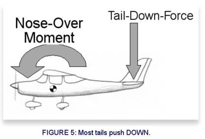
For drag, we use a similar formula where the Cl is replaced by Cd, the so-called drag coefficient. One thing to note; we read the drag coefficient information from a different chart called a Drag Polar. Shown in Figure 4, the Drag Polar illustrates how the drag coefficient varies as a function of the lift coefficient.

Here is the equation for drag:

DRAG = Cd * (0.5) * DENSITY * SPEED * SPEED * AREA

Recall that the Angle-of-Attack is 5 degrees and the lift coefficient is 0.55. Since we know the value of the lift coefficient, we can use the Drag Polar chart shown in Figure 4 to look up the drag coefficient which has a value of roughly 0.0075. Drag coefficients are always shown with four decimal places. When we talk about Drag Coefficients, we consider the ten-thousandths place to be a single Drag Count. For example, the NACA 0012 airfoil shown in Figure 4 has a drag coefficient of seventy-five Drag Counts at the same time that the lift coefficient is 0.55.

Estimating the drag force on our wall-to-wall wing-section model is fairly straight forward. Here is the calculation:

DRAG = Cd * (0.5) * DENSITY * SPEED * SPEED * AREA

DRAG = 0.0075 * (0.5) * 0.002315 * 100 * 100 * 6 = 0.5 pounds.

If we have a real wing which is not infinitely long, we must modify the 2Ddrag coefficient with an additional "3D" term, as shown here:

Cd_3D = Cd_2D + [ Cl * 0.5 / (Pi * e * ASPECT_RATIO)

Cl is the lift coefficient, Pi is 3.14, e is the Oswald Efficiency Factor (use 0.8) and the ASPECT_RATIO is the wingspan divided by average chord length.

PITCHING MOMENT

What about the pitching moment coefficient? The moment is often forgotten by many introductory texts even though it is very important especially for trim drag. For those not familiar with the word “moment”, that is the engineering term for the common word torque.

Remember: Moment is a fancy word for torque.

As a wing flies through the air producing lift, it also has a tendency to create a nose-over moment or torque. In other words, the airfoil wants to flip end over end; often called nosing-over. This is not a desired effect. Some airfoils produce a very strong negative (nose-down) moment and some do not. Most tails push down to counteract the airplanes desire to flip nose over (See Figure 5 below).

History has shown that the (pitching) moment coefficient stays relatively constant when measured about the 25% wing chord position. Because of this, almost all data about airfoil pitching moments are referenced to the 25% chord position. Engineers call this the “Quarter Chord” location. The equation for moment is similar to the lift and drag equations, but it has the actual chord length thrown into it:

PITCHING MOMENT = Cm * (0.5) * DENSITY * SPEED * SPEED * AREA * CHORD

When a pilot lowers his flaps, both the lift and pitching moment increase greatly; the nose-over-tendency is often amplified.

“If that’s true,” I’m often asked, “then why does the nose on my Cessna pitch upward when I drop the flaps?”

This strange effect is caused by two things that happen when we lower the flaps on a high-wing Cessna. The nose-over pitching moment increases greatly, but the flapped wing is also deflecting the trailing air at a much more downward angle. The downward flow of air behind the wing is hitting the horizontal stabilizer at a much steeper angle; an "artificial" angle of sorts. This results in a strong downward lift coefficient on the tail, which essentially pushes the horizontal stabilizer down harder than the wing wants to flip nose down. That’s why the nose pitches up when we drop the flaps on some high wing aircraft.

In Part 4 of this primer series, we will discuss Reynolds Number and laminar flow airfoils.

PART 4:

OZZY REYNOLDS AND HIS NUMBER

You wouldn't give an adult-sized dose of medicine to a baby because the volume is not scaled correctly for their size. A similar thing happens with aerodynamic coefficients. Just because you obtained the coefficients from a small model in a wind tunnel test does not mean they automatically apply to a full-scale aircraft. To ensure that the data obtained from a wind tunnel is applicable to a full-scale aircraft, all we need to do is match Reynolds Numbers. To better explain this concept, let’s go to the aerodynamics laboratory.

We’re now standing next to a wind tunnel. Inside, there's a quarter-scale model of an airplane mounted on a force-measuring device. Let’s call this airplane the Wessna Worrier. The wind tunnel speedometer shows me that the air inside the wind tunnel is traveling at almost 160 miles per hour. I’m just a mediocre pilot, but even I know this airplane could never go that fast. So I ask the operator about this speed discrepancy and he says, “Oh, we’re just trying to match the Reynolds Number to full scale.”

Huh?

The world of engineering is filled with special numbers named after people long gone whom you and I will never meet. One of these people was Osborne Reynolds, an Englishman from the late 1800’s. Mr. Reynolds was obsessed with watching colored dye flow through pipes. He was especially interested in how the dye would start out flowing as a smooth streak (Laminar) and invariably break down into eddy-filled craziness (Turbulent). The same phenomenon can be seen with cigarette smoke rising from an ashtray. Reynolds didn’t know it immediately, but he was really studying the concept of boundary layer growth; a subject that is of paramount importance in aerodynamics. In the absence of boundary layer phenomena, aerodynamics is downright simple. Unfortunately, major things like top-speed and maximum lift are very dependent on boundary layers.

At the beginning of the 20th century, a German researcher named Ludwig Prandtl formulated the equations needed to describe how boundary layers grew. In short, they get thicker and messier as they progress downstream. Prandtl used a subset of the previously known Navier-Stokes equations for his methodology. Very complicated stuff, but Prandtl was a very smart guy.

The thing to know is that the Reynolds Number (Re) contains a summary of flow information. It conveys nearly everything you need to know about a certain flow condition and it doesn’t even have any units. No feet. No inches. No pounds. Nothing. It is a product of the fluid density, fluid velocity, important (characteristic) length, and the reciprocal of the fluids’ viscosity. Think of it as a meat grinder where you pour all the environmental flow conditions in one end and the unitless Reynolds Number plops out the other end.

In essence, when you match the model Reynolds Number with the full-scale Reynolds Number, you are effectively removing the scale effect.

THE SIZE OF YOUR REYNOLDS NUMBER

With a little experience, you can get useful information about a fluid flow just from knowing the magnitude of the Reynolds Number. For example, if you see wind tunnel data taken at Reynolds Numbers of 200,000 or less, it is safe to assume that those airfoils were meant for either model airplanes or high-altitude airplanes; both conditions lead to small Reynolds Numbers. If the data was taken with Reynolds Numbers between about 500K and 6million, it usually applies to general aviation; this is the regime where a lot of historical and freely available wind tunnel data was taken. When the Reynolds Number goes above about 9million, we’re usually talking about fighter jets or passenger airliners. Of course, this is just a rule of thumb and subject to debate.

HOW TO CALCULATE THE REYNOLDS NUMBER:

1. Find out what your velocity is in feet per second. To do this, multiply MPH by 1.4667 or you can multiply KNOTS by 1.689.

2. Find out what your air density is. Remember that this changes with altitude and it must be in slugs per cubic foot. You can use the WingCrafter module in DesignFOIL to find the air density at altitude. For simplicity, 0.002377 slugs per cubic foot is used for a sea level density.

3. Find out the viscosity of air. Use 0.00000037373 (it’s a REALLY small number)

4. Decide what the important dimension is. For wing-sections, that dimension is the chord length. For round objects like spheres, the dimension is the diameter.

Using the above information, use this equation:

REYNOLDS NUMBER = DENSITY * SPEED * DIMENSION / VISCOSITY

The equation is very telling - the numerator (top portion) is made up of momentum effects and the denominator (bottom portion) is made up of viscosity effects. As a Reynolds Number grows larger, it implies that the momentum effects of the fluid are becoming more important that the viscosity effects.

If you’d rather avoid the above math, here’s a simplified formula for sea level Reynolds Number using mph and feet:

REYNOLDS NUMBER = 9360 * SPEED(in mph) * DIMENSION (in feet)

The mention of Reynolds Number implies "the appropriate use of a given set of wind tunnel data." It’s easy to think that any coefficient data that you get from a wind tunnel applies to the full-scale airplane at the same speed. As we've learned, though, the coefficient data is only “good” for the Reynolds Number that it was taken at. So, to get full-scale Reynolds Number data from a wind tunnel, you have to increase the airspeed over the model in an effort to match what would be the Reynolds number on a full scale model.

For example, to obtain aerodynamic coefficient data ( Cl, Cd, Cm ) from a half-scalemodel that is applicable to the full-scale aircraft, we would have to double the airspeedover the model in an effort to equate the Reynolds Numbers. Or we could double our air density instead, but that is very expensive and difficult to do. So in summary, if we cut the wing chord in half, the Reynolds number also gets cut in half. To compensate, we’d have to double the airspeed to keep the same Reynolds Number. It can be very confusing sometimes.

Reynolds Number Anecdote (It's true!)

A friend of mine once tested an Estes model rocket in a slow wind tunnel. Because the actual rocket was so small and our wind tunnel so slow, he instead built a giant "model" of the rocket that was ten times LARGER than the real rocket. At that scale, he could slow the airspeed in the wind tunnel to one-tenth the speed that the rocket really flies at; this method gave him identical Reynolds Numbers. Therefore, he could apply the Cl and Cd values that he got from the wind tunnel directly to his flight performance estimates, even though the model size was very different.

A TECHNIQUE FOR REDUCING DRAG

Stories come and go about the legendary airfoils on the WWII era P51 Mustang. It is often said that the airplane’s high speed was a result of its so-called “laminar flow” airfoils which you are about to learn about. While it is true that the wing drag was probably less than contemporary aircraft of the time, the metal construction at the time prevented those airfoils from reaching their full potential regarding drag reduction. One of the larger contributors to the extreme speed was probably the enormous power from the Merlin engine.

Methodically-developed laminar flow airfoils have been around since even before WWII; they were the brain child of Eastman Jacobs, an engineer at the NACA during the 1930’s. In the preceding 30 years, smart people like Germany's Ludwig Prandtl learned that drag could be reduced by controlling the shape and growth-rate of the layer of thin fluid just above the wing surface. This region of fluid became known as theboundary layer because it was the boundary between the wing surface (airspeed = zero) and the outside freestream (airspeed = not zero).

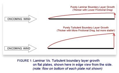
For the following explanation, refer to Figure 1 which shows the two common types of boundary layer growth on a flat plate.

The viscosity of air, or its' "gooeyness", plays a very important role in the thin region of air just above the surface of any moving object. On a microscopic level, even the most polished surface still looks like a mountain range. Air molecules that try to maneuver these peaks often get stuck and donate their momentum to the mountains themselves (i.e. the wing) in the form of heat and friction. Just prior to being halted by the surface of the wing, these molecules of air had been moving at the speed of the aircraft. The speed changes from full aircraft speed to zero over a tiny distance.

On a larger scale this effect is felt as a friction force tugging on the wing surface (i.e. drag). Again, the velocity of the air in direct contact with the wing is zero. As we move away from the surface, the speed of the air accelerates quickly to match that of the freestream flow. Because this extreme acceleration takes place over a height of just a few millimeters, the viscosity of air is very important.

A good way to picture this is to envision traffic on a seven-lane freeway in Los Angeles. The far-right lane is where cars are entering and leaving the traffic flow. They are moving slowly and may even be stopped. As you change lanes away from the slow lane, the traffic moves faster and faster until you reach the fast lane where the car velocities are highest, hardly affected by the slow lanes at all.

At first, the velocity-change between the bottom and top of the boundary layer is done smoothly and produces a small amount of friction drag on the airfoil. The layers of air in the boundary layer flow smoothly over one another without any swirling. This type of boundary layer is called Laminar and produces very little friction. Think of it as a stack of highly polished playing cards being dragged over carpet. The cards glide effortlessly over each other while the bottom cards are left behind. 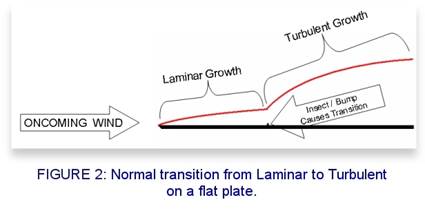The trade-off is that this low-friction laminar boundary layer is not very stable and will switch to a draggier, yet more stable, turbulent boundary layer at the slightest hint of a surface imperfection which trips the laminar flow. And in the real world, the boundary layer usually starts out laminar and transitions to turbulent as shown in Figure 2 below.

The boundary layer growth on an airfoil is more complicated than a flat plate. The difference, shown in Figure 3, is in what causes transition to occur. Imperfections will still trip the laminar boundary layer, but airfoils have the additional phenomenon of the pressure gradient. The pressure gradient refers to how the pressure is changing as we march downstream from the nose of the airfoil. If the pressure gradient is negative, we feel like we are being swept along faster and faster (like a canoe being pulled toward a waterfall). When the pressure gradient is positive, we feel higher and higher pressure and a certain feeling of "pushback" from the air as we march downstream (like that same canoe going from a high-speed river into a calm lake).

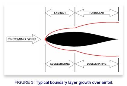
On the forward portion of an airfoil, the pressure gradient is negative and the air is accelerating downstream; a perfect habitat for a laminar boundary layer. However, when the air stops accelerating and begins decelerating, we get a positive pressure gradient. That causes the laminar boundary layer to transition to a turbulent boundary layer. The flow loses its smoothness and starts filling with eddies, causing the outside air to start mixing with the already formed boundary layer. This “turbulent” portion of the boundary layer is thicker and produces relatively higher friction drag compared to the smooth laminar portion of the boundary layer.

The following list of steps outlines the general birth and death of a boundary layer on an airfoil:

1. The oncoming air slams into the leading edge and stops. This point (shown as a red dot in Figure 3) is called the Stagnation Point. This location serves as a dividing line. The air beneath goes below the airfoil. The air above the Stagnation Point goes over the top of the airfoil.

2. As the airflow leaves the Stagnation Point, it accelerates past both the upper and lower surfaces due to the strong negative pressure gradient. This unique flow forms a laminar boundary layer. It continues to grow in a laminar fashion until the minimum pressure (max velocity) is reached. Unless previously tripped by a surface imperfection, this is the likely transition point.

3. After transition, the boundary layer becomes turbulent, eventually leaving the airfoil at the trailing edge.

There are a few known variants to this script. If the flow condition is at a very low Reynolds Number, the laminar boundary layer sometimes skips the transition-to-turbulent phase and instead separates, never to be heard from again! Sometimes it immediately reconnects forming a thicker turbulent boundary layer than normal. The region between the laminar separation and the turbulent re-connection looks like a bubble and is often called a Laminar Bubble. If the laminar bubble fails to re-establish a viable turbulent boundary layer, the air just leaves the airfoil at that point and the wing flies around in a semi-stalled condition.

If you've done any radio-controlled airplane flying, you may have seen airplanes with zig-zag tape on the upper surface of the wing. The purpose of such a boundary layer tripping device is to combat the laminar bubble problem that occurs at model flight scales. Those pilots are taking matters into their own hands and forcing that sensitive laminar boundary layer flow to trip itself into a more stable turbulent boundary layer (to avoid separation). After all, a draggy turbulent layer is better than separation and stall.

Using trip devices (trip strips, vortex generators, etc...) can force an otherwise laminar bubble to stay attached to the wing long past it's normal stall angle - turbulent boundary layers tend to be "stickier" than laminar boundary layers. Some academic cargo-payload competitions can benefit from this effect by flying at higher Angles-of-Attack, thus carrying more weight than just a clean wing.

Keep in mind that the boundary layer thicknesses depicted in Figure 3 are greatlyexaggerated. Here is what you can expect in the real world: say you are flying along at 100knots at sea level staring at the pretty sailboats. Your airplane's wing has a 5-foot (152cm) chord. The airfoil design consistently produces laminar airflow over the first 20% of the surface, with the rest being turbulent. The laminar boundary layer thickness would be about 0.060" (1.5mm). The turbulent boundary layer thickness could grow from 3/8" to 1/2" (9.5-13mm) at the trailing edge of the wing.

Over the years, we have discovered that creating and maintaining laminar boundary layers is much trickier in real life. Unlike the mirror finishes of wind tunnel models, real airplanes are very dirty. Have you ever seen the leading edge of a wing from a full-scale airplane? It is coated with insect guts - laminar flows don't like insect guts.

In Part 5 of this primer series, we will discuss laminar flow airfoils in detail.

Chapter 5

LAMINAR FLOW, BY ACCIDENT

During the 1930’s a self-taught aerodynamicist named David R. Davis went to the trouble of patenting an airfoil design, which he called the “Fluid Foil” (US Patent #1,942,688). He considered his design special because it exhibited lower drag than most other common airfoils, but he wasn’t sure why. His timing was impeccable because fortunately for Mr. Davis, the Consolidated Aircraft Company was looking for a marketing trick to make their new aircraft stand out from the competition; a unique low-drag wing was just the ticket. After verifying the low-drag performance of the Fluid Foil in a wind tunnel, Consolidated licensed the airfoil patent from Mr. Davis in 1937. The Fluid Foil eventually found its way into the wing design of the B-24 Liberator bomber during WW2. (Ref: Vincenti, 1990)

Without knowing it, Mr. Davis had inadvertently invented the first airfoil to achieve low-drag through encouragement of a laminar boundary layer, the rarely seen smooth airflow that briefly exists before the higher-drag, turbulent boundary layer takes over. The concept of the laminar boundary layer was discussed in detail in Part 4 of this airfoil primer series.

Consolidated Aircraft went on to build over 19,000 of the B-24 bombers, putting it ahead of the venerable B-17 in production count. Although many people consider the P-51 Mustang to be the first aircraft to use laminar flow airfoils, the truth is that the B-24 was the first, albeit accidental, aircraft to use laminar flow airfoils. The true significance of the P-51 wing was that it was the first to intentionally use the new scientifically developed NACA 6-series laminar flow airfoils.

As interesting as these historic facts are, it’s even more amazing to learn that neither of these airfoils actually produced much usable laminar flow when finally integrated on real world aircraft. In fact, they were probably just as turbulent as every other plain vanilla airfoil out there. We can forgive the designers though - it's one thing to base all of their data on finely polished wind tunnel models and it's another thing to build real wings out of sheet metal, rivets, bucking bars, hammers... all with a war raging against them. Add mosquito guts onto the leading edges and they had little chance of establishing much of a laminar boundary layer at all.

I don’t mean to downplay the development of laminar flow airfoils on metal aircraft. Analytically, it was a significant leap for the early engineers to "backward-solve" the formulas used for analyzing airfoils. Rather than starting with known surface coordinates and calculating the resulting pressure distribution, the NACA personnel figured out how to take the desired pressure distribution and back out the required surface contours!

Due to modern day construction methods, stiff composite materials, and improved laminar flow airfoil designs, there is renewed interest in the use of laminar flow airfoils in general aviation. Most modern racing aircraft (such as the decambered NASA NLF used on Nemesis NXT) use some type of laminar flow airfoil; often modified for proprietary purposes.

Laminar Or Not?

It may surprise you to learn that all airfoils have some laminar flow; even the airfoil used on the Wright Flyer. Granted, the laminar flow on the Wright Brothers airplane only lasted a few percent of the chord length, but there was some laminar flow. This brings up the question of how to classify airfoils. Laminar or not laminar? As it turns out, the answer is subjective.

Generally speaking, for an airfoil to be considered a laminar flow airfoil, it must have a favorable pressure gradient that extends past 30% of the chord length. Laminar boundary layers are sensitive beasts and prefer to have the surface pressurecontinuously dropping as they march downstream from the leading edge. When the surface pressure stops dropping and begins to increase instead, the smooth laminar flow becomes turbulent, fighting its way to the trailing edge. It’s easier to fall down a hill than walk back up it again.

Figure 2 (below) shows a series of very common airfoils and how much of their chord length will experience favorable pressure gradients (i.e. laminar boundary layers) under ideal conditions. It is important to understand that extensive laminar flow is usually only experienced over a very small range of angles-of-attack, on the order of 4 to 6 degrees. Once you break out of that optimal angle range, the drag can increase by as much as 40% depending on the airfoil.

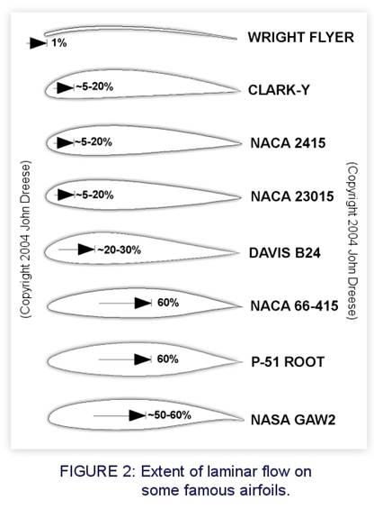
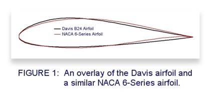
Look closely at the airfoils in Figure 2. The laminar designs in the lower half exhibit extensive laminar flow (past 50%). They generally have sharper noses which can result in a more unpredictable and sharp stall. However, the most obvious trait is therearward placement of the maximum thickness. If you look at a wing edge-on and notice that the maximum thickness is far back, you can bet that the airfoil is a laminar flow airfoil. I recommend that you look at a Piper Tomahawk wing edge-on; you’ll discover right away that it uses a GAW airfoil.

The Quest for Low Drag

To understand the great advantages of laminar flow airfoils, we need an experiment. Imagine that we point a sheet of plywood into a 70 mph air stream with no angle between the chord length and the relative wind (zero degrees angle of attack). If we could magically force the boundary layer to stay 100 percent laminar from leading edge to trailing edge, the frictional drag force would be roughly 0.6 pounds (0.3 Kg). Now, if we flipped a switch to make the boundary layer completely turbulent, the frictional drag force would jump to almost 3 pounds (1.4 Kg), a net rise in drag of nearly 500 percent!

As we can see from our simple plywood airfoil example, laminar boundary layers result in much less wing surface friction compared to a turbulent boundary layer. Remember that real world wings have a mixture of laminar and turbulent boundary layers so the actual gains are on the order of 40 to 50 percent. The ultimate goal of a laminar flow airfoil is one where we try to maximize the laminar boundary layer while minimizing the turbulent boundary layer without making the whole thing too overly sensitive to surface finish.

Consider the builder’s ability to control the wing contour during construction and flight. The surfaces of metal airplanes tend to “oilcan” during flight and this can change the contour enough to trip the laminar boundary layer.

When using composites, it’s important to keep close tolerances on the airfoil contour. Contour control of a surface isn’t just a step-height allowance; it depends on the chord length that it occurs over. Aluminum? That's a tough challenge.

Speaking of surface finish, I’ve heard stories of sailplane flyers actually scuffing the gloss off their wings in a chord-wise direction from leading edge to trailing edge with 600-grit sandpaper. If roughing up a surface reduces drag, that typically means that the boundary layer was blowing off prematurely or had laminar bubble issues; roughing up the surface helps both of those situations (in some ways, it is similar to why dimples reduce drag on a golf ball). Those problems are usually only experienced at very low Reynolds Numbers (small chord wings flying at either slow speeds or high altitudes).

Anecdotal stories of Indy race car guys rubbing baby powder on their cars to make it more “slippery” have been circulating in the pits for years. The baby powder may have felt smoother to their fingertips, but not to the air molecules! Traditionally, a very smooth, clean, and highly polished surface will always result in lower drag numbers. Wax it, don’t powder it!

Designing the Perfect Airfoil

You may be thinking the same thing that NACA engineer Eastman Jacobs thought back in the 1930’s. Why not design airfoils that only produce laminar boundary layers? That way, you could have ultra low wing drag. Let’s take a look at the numbers.

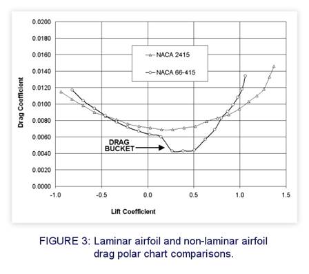
We can quantify the reduction in drag due to laminar boundary layer development. Figure 3 shows the reason why engineers have chased after laminar flow airfoils for so long. This graph compares the drag polars of two airfoils. One is for a typical airfoil (NACA 2415) and the other is for a laminar flow airfoil (66-415). For the latter airfoil, we see that the drag coefficient drops noticeably between a lift coefficient of roughly 0.25 and 0.5. Your goal, as a designer, is to make sure that your desired cruise lift coefficient falls somewhere in that drag bucket. (See arrow in Figure 3)

Let’s briefly recall what a boundary layer is from Part #4 of the Airfoil Primer series. Even the smoothest surface looks like a mountain range when viewed on a microscopic scale. As air flows past, hugging these surfaces, some of the molecules get stuck and donate their energy to the microscopic mountains themselves. These molecules of air that were originally moving with the speed of the oncoming air flow are halted and brought to zero velocity right at the surface! In engineering, this is called the “no-slip” condition. On a larger scale this effect is felt as a friction force tugging at the wing surface.

We can break it down even further. When the boundary layer begins forming at the leading edge, it is flowing smoothly with each microscopic layer of air flowing easily over the next like a deck of waxed playing cards sliding over one another. This portion of the boundary layer produces very little drag force, but unfortunately it only lasts until the air racing back along the airfoil begins to slow down. With non-laminar airfoils, this typically happens within five to twenty percent of the chord length. At that point, the laminar boundary layer will begin mixing with outside air and become filled with small eddies. These so-called turbulent boundary layers can be surprisingly stable, but the trade-off is they produce higher drag than the laminar boundary layers do.

Bubble Trouble

Prior to now, you’ve learned that all laminar boundary layers grow up to become turbulent boundary layers. When operating at very low Reynolds Numbers (less than 100,000 for example), this transition to turbulent sometimes does not occur. The boundary laminar boundary layer encounters the increasing pressure and occasionally explodes away from the surface, never to be heard from again. Sometimes it immediately reconnects forming a much thicker turbulent boundary layer than normal. The region between the laminar separation and the turbulent re-connection points looks like a bubble and is often called a Laminar Bubble. If the laminar bubble fails to stay connected, the boundary layer leaves the airfoil at that point and the wing flies around in a semi-stalled condition. This is very bad. There have been a few rare cases where airfoils utilizing extreme laminar flow have been so sensitive that even raindropscaused the boundary layer to become unstable and blow off the surface, causing a stall.

You may have seen radio controlled airplanes with zigzag tape on the upper surface of the wing to combat these low Reynolds Number problems. Those pilots are taking matters into their own hands and forcing that sensitive laminar flow to trip itself into a turbulent boundary layer before separating. After all, a guaranteed turbulent boundary layer is better than a chance of separation and stall. Some folks have used this trick to get their radio-controlled airplanes to carry more weight than normal during cargo-carrying contests (hint, hint).

Luckily, this tendency to go from laminar directly to separated occurs less often as the Reynolds number is increased.

Key points to remember about boundary layer development:

1. Laminar boundary layers prefer air that is accelerating (lowering pressure), but will convert to turbulent the instant the air begins to slow down. Laminar means LOWER DRAG.

2. Turbulent boundary layers will form from a laminar boundary layer once the air begins slowing down. Turbulent means HIGHER DRAG, but not terrible drag. In the case of a golf ball, the turbulent boundary layer actually reduces drag!

3. At very low Reynolds Numbers, you may experience the draggy effect of laminar bubbles.

The Final Laminar (Plot) Twist

In yet another twist regarding laminar flow airfoils on metal aircraft, they turned out to be excellent performers for high-speed aircraft. High-speed, as in jet-aircraft. And it had nothing to do with laminar boundary layers; rather it was a function of moving the minimum pressure location significantly behind the leading edge. This resulted in an increased critical Mach number, which allowed jet-fighters to go a little bit faster by minimizing supersonic drag over the wings (even a subsonic airplane can experience pockets of supersonic airflow on top of the wing due to local accelerations).

You probably don’t have a jet engine though. So how can you make good use of laminar flow airfoils? First of all, if you’re building a sheet metal wing and won’t be flying past Mach 0.6 (about 450 mph), then don’t bother with extreme laminar flow airfoils. Conventional NACA airfoils will work just fine for your purposes. Van’s Aircraft has used the NACA 5-digit series very effectively on their RV models.

However, if you are building a stiff composite wing, you may want to use a NACA 6-series or one of the more modern NASA natural laminar flow airfoils. Just be sure to keep those leading edges clean.

The next time you visit Oshkosh, Sun-N-Fun, or the Reno Air Races, look at the wings edge-on and try to guess if they are using a laminar flow airfoil. Ask the pilot about it; they will appreciate that you noticed.

Congratulations

You've reached the end of the five-part Airfoil Primer series. Let me know if these have helped you.

Recommended References:

1. Theory Of Wing Sections: Including a summary of airfoil data, Abbott and von Doenhoff, Dover Publications, ISBN 0-486-60586-8.

2. The Illustrated Guide To Aerodynamics, Hubert “Skip” Smith, 1985, Tab Books, ISBN 0-8306-2390-6

3. Airfoil Selection, Barnaby Wainfan, self-published and available from EAA.

4. Basic Wing & Airfoil Theory, Alan Pope, 1951, McGraw-Hill Book Company (does not have ISBN number).

5. History of Aerodynamics, John D. Anderson Jr., 1998, Cambridge University Press, ISBN 0-521-66955-3

6. What Engineers Know and How They Know It, Walter Vincenti, 1990, Johns Hopkins University Press, ISBN 0-8018-4588-2

ABOUT THE AUTHOR

John Dreese is the creator of the DesignFOIL airfoil creation and analysis software package, available at:

www.dreesecode.com

If you have any comments or questions, please feel free to email John at:

DesignFOIL@gmail.com

Twitter:

http://www.twitter.com/JJDreese/