You wouldn't give an adult dose of medicine to a baby because the volume is not appropriately scaled for them. A similar thing happens with aerodynamic coefficients. Just because you obtained the coefficients during a wind tunnel test does not mean they automatically apply to a full-scale aircraft. To ensure that the data obtained from a wind tunnel is applicable to a full-scale aircraft, all we need to do is match Reynolds Numbers. To better explain this concept, let’s go back to the wind tunnel.

We’re now standing next to the wind tunnel. Inside the tunnel there is a quarter-scale model of an airplane mounted on a force-measuring device. Let’s call this airplane the Pessna Worrier. The wind tunnel speedometer tells me that the air inside the wind tunnel is traveling at almost 160 miles per hour. Although I’m just a mediocre pilot, I know this airplane could never go that fast. So I ask the operator about this speed discrepancy and he says, “Oh, we’re just trying to match the Reynolds number to full scale.”

Huh?

~flashback~

The world of engineering is filled with special numbers named after people long dead whom you and I will never meet. One of these people was Osborne Reynolds, an Englishman from the late 1800’s. Mr. Reynolds was obsessed with watching colored dye flow through pipes. He was especially interested in how the dye would start out flowing as a smooth streak (Laminar) and invariably break down into eddy-filled craziness (Turbulent); the same phenomenon can be seen with cigarette smoke rising from an ashtray. Reynolds didn’t know it, but he was really studying the concept of boundary layer growth; a subject that is of paramount importance in aerodynamics. In the absence of boundary layer phenomena, aerodynamics is downright simple. Unfortunately, major things like top-speed and maximum lift are very dependent on boundary layers.

At the beginning of the 20th century, long after Osborne Reynolds, a German researcher named Ludwig Prandtl formulated the equations needed to describe how boundary layers grew. In short, they get thicker and messier as they progress downstream. Prandtl used a subset of the previously known Navier-Stokes equations for his methodology. Very complicated stuff, but Prandtl was a very smart guy.

The thing to know is that the Reynolds Number (Re) contains a summary of flow information. It conveys nearly everything you need to know about a certain flow condition and it doesn’t even have any units. No feet. No inches. No pounds. Nothing. It is a product of the fluid density, fluid velocity, important length, and the reciprocal of the fluids’ viscosity. Think of it as a meat grinder where you pour all the environmental flow conditions in one end and the unitless Reynolds Number plops out the other end.

In essence, when you match the model Reynolds Number with the full-scale Reynolds Number, you are matching the viscous effects of the two flow conditions. You are removing the scale effect.

With a little experience, you can get useful information about a fluid flow just from knowing the magnitude of the Reynolds Number. For example, if you see wind tunnel data taken at Reynolds Numbers of 200,000 or less, it is safe to assume that those airfoils were meant for either model airplanes or high-altitude airplanes; both conditions lead to small Reynolds Numbers. If the data was taken with Reynolds Numbers between about 500K and 6million, it usually applies to general aviation; this is the regime where most of the wind tunnel tests are run. When the Re goes above about 9million, we’re usually talking about fighter jets or passenger airliners. Of course, this is just a rule of thumb and subject to debate.

HOW TO CALCULATE THE REYNOLDS NUMBER:

• 1) Find out what your velocity is in feet per second. To do this, multiply MPH by 1.4667 or you can multiply KNOTS by 1.689.
• 2) Find out what your air density is. Remember that this changes with altitude and it must be in slugs per cubic foot. You can use the WingCrafter module in DesignFOIL to find the air density at altitude. For simplicity, 0.002377 slugs per cubic foot is used for a sea level density.
• 3) Find out the viscosity of air. Use 0.00000037373 (it’s a REALLY small number)
• 4) Decide what the important dimension is. For wing-sections, that dimension is the chord length. For round objects like spheres, the dimension is the diameter.

Using the above information, use this formula:

If you’d rather avoid the above math, here’s a simplified formula for sea level Reynolds Number suggested by my friend Neal Willford:

The mention of Reynolds Number implies "the appropriate use of a given set of wind tunnel data." It’s easy to assume that any coefficient data that you get from a wind tunnel applies to the full-scale airplane at the same speed. As we've learned, though, the coefficient data is only “good” for the Reynolds Number that it was taken at. So, to get full-scale Reynolds Number data from a wind tunnel, you have to increase the airspeed over the model in an effort to match what would be the Reynolds number on a full scale model.

For example, to obtain aerodynamic coefficient data ( C_l, C_d, C_m ) from a half-scale model that is applicable to the full-scale aircraft, we would have to double the airspeed over the model in an effort to equate the Reynolds Number. Or we could double our air density instead, but that is very expensive and difficult to do. Just remember that if we cut the wing chord in half, the Reynolds number also gets cut in half. To compensate, we’d have to double the airspeed to keep the same Reynolds Number. It can be very confusing sometimes.

Reynolds Number Anecdote (It's true!)
A friend of mine once tested an Estes model rocket in a slow wind tunnel. Because the actual rocket was so small and our wind tunnel so slow, he instead built a giant "model" of the rocket that was ten times LARGER than the real rocket. At that scale, he could slow the airspeed in the wind tunnel to one-tenth the speed that the rocket really flies at; this method gave him identical Reynolds Numbers. Therefore, he could apply the C_l and C_d values that he got from the wind tunnel directly to his flight performance estimates, even though the model size was very different.

Stories come and go about the legendary airfoils on the WWII era P51 Mustang. It is often said that the airplane’s high speed was a result of its special low-drag “laminar flow” airfoils which you are about to learn about. While it is true that the wing drag was probably less than similar aircraft, the metal construction at the time prevented those airfoils from reaching their full potential regarding drag reduction. It’s more likely that the extreme speed was a result of the enormous power from the Merlin engine.

Methodically developed laminar flow airfoils have been around since even before WWII; they were the brain child of Eastman Jacobs, an engineer at the NACA during the 1930’s. In the preceding 30 years, smart people like Germanys’ Ludwig Prandtl learned that drag could be reduced by controlling the shape and growth-rate of the boundary layer; a thin layer of slower moving air that coats all moving objects.

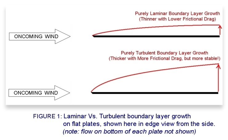
For the following explanation, refer to Figure 1 which shows the growth of boundary layers on a flat plate.

In the region of air very close to the surface of any solid object the viscosity, or gooeyness, of air plays a big role. On a microscopic level, even the smoothest surface looks like a mountain range. Air molecules that try to maneuver these peaks often get snagged and donate their momentum to the mountains themselves in the form of heat and friction. So these molecules of air that were originally moving with the speed of the oncoming flow are halted and brought to zero velocity right at the surface! On a larger scale this effect is felt as a friction force applied to the wing surface. The velocity of the air in direct contact with the wing is zero. As we move away from the surface, the speed of the air accelerates quickly to match that of the freestream flow. Because this extreme acceleration takes place over a height of just a few millimeters, the viscosity of air is very important.

A good way to picture this is to envision traffic on a seven-lane freeway in Los Angeles. The far-right lane is where cars are entering and leaving the traffic flow. They are moving slowly and may even be stopped. As you move away from the slow lane, the traffic moves faster and faster until you reach the fast lane where the car velocities are hardly affected by the slow lanes.

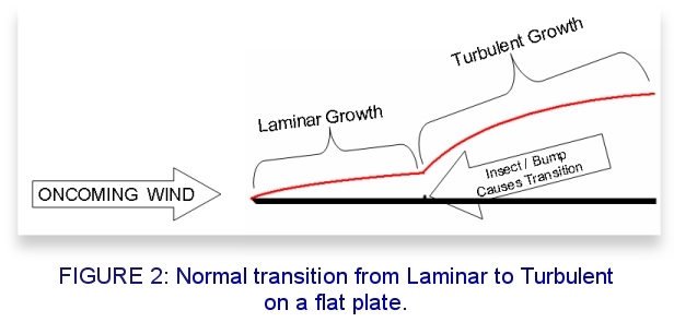
At first, the velocity-change between the bottom and top of the boundary layer is done smoothly and produces a small amount of friction drag on the airfoil. The layers of air in the boundary layer flow smoothly over one another without any swirling. This type of boundary layer is called Laminar and produces very little friction. The tradeoff is that this low-friction laminar boundary layer is not very stable and will switch to a draggier yet stable turbulent boundary layer at the slightest hint of a surface imperfection which trips the laminar flow. And in the real world, the boundary layer usually starts out laminar and transitions to turbulent as shown in Figure 2.

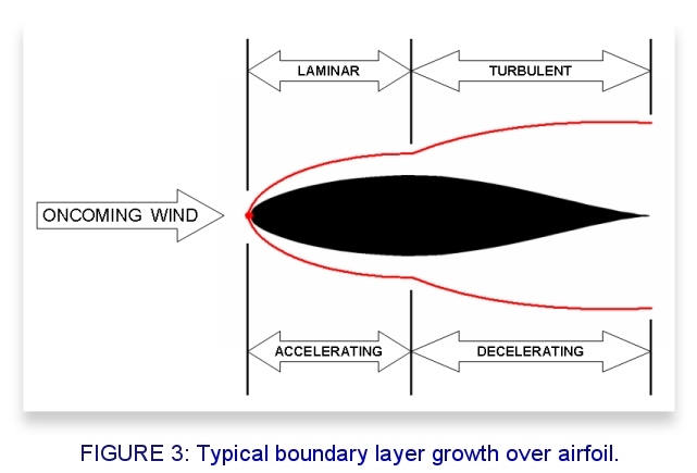
The boundary layer growth on an airfoil is more complicated than a flat plate. The difference, shown in Figure 3, is in what causes transition to occur. Imperfections will still trip the laminar boundary layer, but airfoils have the additional phenomenon of the pressure gradient. The pressure gradient refers to how the pressure is changing as we march downstream. If it is negative, we feel like we are being swept along faster and faster. When the pressure gradient is positive, we feel higher and higher pressure and a certain feeling of "pushback" from the air as we march downstream.

On the forward portion of an airfoil, the pressure gradient is negative and the air is accelerating downstream; a perfect habitat for a laminar boundary layer. However, when the air stops accelerating and begins decelerating, we get a positive pressure gradient. That causes the laminar boundary layer to transition to a turbulent boundary layer. So the flow loses its smoothness and starts filling with eddies; causing the outside air to start mixing with the already formed boundary layer. This “turbulent” portion of the boundary layer is thicker and produces relatively higher friction drag compared to the smooth laminar portion of the boundary layer.

Generally, here is how a boundary layer develops on an airfoil. Please refer to Figure 3 (above) while following these steps:

• 1) The oncoming air slams into the leading edge and stops. This point (shown as a red dot) is called the Stagnation Point.
• 2) From there the boundary layer grows laminarly over both the upper and lower surfaces until the minimum pressure (max velocity) is reached. Unless previously tripped by a surface imperfection, this is the likely transition point.
• 3) After transition, the boundary layer becomes turbulent before it eventually leaves the airfoil at the trailing edge.

There are some variations to this script. If the flow condition is at a very low Reynolds Number, the laminar airflow sometimes skips transitioning to turbulent and simply separates never to be heard from again! Sometimes it immediately reconnects forming a thicker turbulent boundary layer than normal. The region between the laminar separation and the turbulent reconnection looks like a bubble and is often called a Laminar Bubble. If the laminar bubble fails to re-establish a viable turbulent boundary layer, the air just leaves the airfoil at that point and the wing flies around in a semi-stalled condition.

You may see radio controlled airplanes with zig-zag tape on the upper surface of the wing to combat this problem. Those pilots are taking matters into their own hands and forcing that sensitive laminar flow to trip itself into a more stable turbulent boundary layer (to avoid separation). After all, a draggy turbulent layer is better than separation and stall! Some folks have used this trick to get their RC planes to carry more weight than normal.

Keep in mind that the boundary layer thicknesses depicted in Figure 3 are greatly exaggerated. Here is what you can expect: say you are flying along at 100knots at sea level gazing at the pretty sailboats. Your airplane's wing has a 5-foot (152cm) chord. The airfoil design consistently produces laminar airflow over the first 20% of the surface, with the rest being turbulent. The laminar boundary layer thickness would be about 0.060" (1.5mm). The turbulent boundary layer thickness would grow to 3/8" - 1/2" (9.5-13mm) at the trailing edge of the wing.

Over the years, we have discovered that creating and maintaining laminar boundary layers is much trickier than it seems. Unlike the mirror finishes of wind tunnel models, real airplanes are very dirty and laminar flow is very sensitive to imperfections and hard to achieve. Have you ever seen the leading edge of a general aviation airplane? It is coated with insect guts and laminar flows just don't like that.

In the next part, we will discuss the ins and outs of laminar flow, and what we can realistically expect from a wing.

NOTE: DesignFOIL Standard Edition is on sale for only $29 right now.

Now to read about the secrets of laminar flow airfoils...